Article 2-1
|
|
1) The market is an oligopoly at the outset.
2) There are two suppliers, a cost-efficient leader, often called "Top Dog", and a cost-inefficient follower (the follower). 3) Decisions are made in sequence. |
The first condition at the outset would suggest a colluded price, under which a cartel profit margin is fatter than competitive profit in the case of an open market. This condition allows suppliers to exert pricing power by undertaking under-production via collusion. In other words, it would require a very unusual reason, one with more importance than profit margin, for oligopolies to initiate over-production to breach their profit margins.
The second condition states that the top dog has a fatter insulation of profit margin than the follower does.
The third condition, together with the previous one, could create a motive for the top dog to deter its competitor’s market share advancement. It can be achieved effectively by initiating over-production within its own insulation of fatter profit margin in an attempt to damage the profit margins of the follower. While sacrificing its own profit margin until it finally defeats the competitor, as its market share expands, it should expect the total profit ( = profit margin × sales volume) to increase higher than ever: otherwise, this strategy would not make any economic sense, therefore, should be avoided.
Prior to waging the deterrence game, the top dog has to command an ex-ante medium-term expectation about the follower’s response. The top dog has to be convinced that under the given conditions, the strategy would not give the follower any other choice but to follow the leader’s intended alternative: either to scale back or to exit from the operation in the medium to long term. Moreover, in order to better position itself in commanding the game and coercing the follower to engage in the anticipated response, the top dog has to provoke pronounced action in order to unequivocally communicate to the market the credibility of its commitment on its over-production initiative.
In a nutshell, it is imperative that a depressed price level be pronounced for the success of the deterrence game; furthermore, the lower price needs to last as long as the game continues. However, the game only continues as long as the follower persists. Therefore, the effectiveness of the strategy is woven into the time horizon as well as the price level. As a result, the less time it takes to conclude the game, the shorter-lived a depressed price level, therefore, the less costly the strategy. The longer time it takes to conclude the game, the longer-lived a depressed price level, therefore, the costlier the strategy. However, if the top-dog has under-estimated the ability of the follower, the result will be detrimental to both. Neither will benefit from the game within the supply space, while the demand side would benefit from the cost deflation.
In brief, the strategy outlined above in which decisions are made sequentially gives the leader a first-mover advantage, meaning the leader’s initiative would “force the follower to scale back its production or even punish or eliminate” the cost-disadvantaged competitor (Pintos and Piros, 2013, p176). However, it also creates great uncertainty in the success of the game when the top dog miscalculates the ability and resilience of the new entrant competitors.
Historical analogy:
the recurrence of precedence
In this section, we will review Kaletsky’s analogy over those two analogous events along the historical price chart. Chart A traces the trajectory of crude oil prices both in nominal and in real terms (2014 USD). Along the inflation-adjusted price chart, Kaletsky portrayed the real price level at $50 (2014 USD term) as a demarcation line between oligopoly and open competitive markets. The red dotted line in the chart identifies the $50 real price demarcation line that Kaletsky contemplated.
The reference point of the real price at $50 (2014 USD term) was derived from the 1985 historical precedent of the crude oil market regime shift. OPEC has exerted its cartel power since the Iranian revolution in 1979. However, in 1985, OPEC abandoned its cartel power and waged a deterrence game against the late entrants. During this period, between 1979 and 1985, the real price exceeded the $50 real price demarcation line. After 1985, the real price breached the $50 real price demarcation line, and over next 20 years, remained below the $50 real price demarcation line with rare exceptions. Based on this technical observation, Kaletsky suggested that the $50 real price (2014 USD term) might be a possible demarcation line between the oligopoly regime and the competitive market regime.
The reference point of the real price at $50 (2014 USD term) was derived from the 1985 historical precedent of the crude oil market regime shift. OPEC has exerted its cartel power since the Iranian revolution in 1979. However, in 1985, OPEC abandoned its cartel power and waged a deterrence game against the late entrants. During this period, between 1979 and 1985, the real price exceeded the $50 real price demarcation line. After 1985, the real price breached the $50 real price demarcation line, and over next 20 years, remained below the $50 real price demarcation line with rare exceptions. Based on this technical observation, Kaletsky suggested that the $50 real price (2014 USD term) might be a possible demarcation line between the oligopoly regime and the competitive market regime.
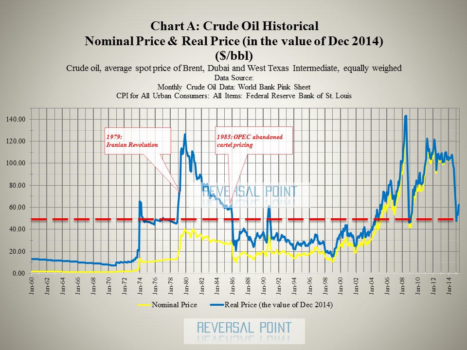
Between 2005 and 2014, with the exception of the aftermath of the Global Financial Crisis in late 2008, the real price restored its high collusion power and remained beyond the $50 real price demarcation line. In 2014, when OPEC refused to reduce production in response to demand softening, the price plunged and the real price breached the demarcation line. This is analogous to the 1985 case in which OPEC abandoned the cartel collusion pricing in order to shift its strategy to take back the market share from its competitors. (Kaletsky, 2015, January 14)
Chart B, superimposing the historical volume of the crude oil production along the real price of crude oil, confirms Kaletsky’s remark about the precedent in 1985 from a volume perspective.
Chart B, superimposing the historical volume of the crude oil production along the real price of crude oil, confirms Kaletsky’s remark about the precedent in 1985 from a volume perspective.
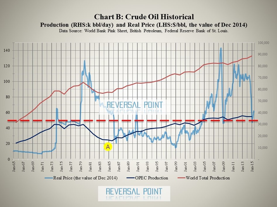
After the price hike in 1973, as OPEC maintained its volume of production on hold from 1974 to 1979, the real price remained plateaued. The production control power of the cartel to influence the price is visually confirmed on this chart.
However, after skyrocketing due to the Iranian Revolution in 1979, the real price reversed its momentum in 1980. The graph illustrates that the past two-step price hike— the first in 1974 and the second in 1979—had already impaired the existing demand mechanism. What is apparent from Chart B is that since 1980, despite its further effort to reduce the volume, OPEC failed to contain the price decline. Although having managed to defend the pre-1979 price level until 1984, OPEC shifted its strategy in 1985 after confirming the continuation of the price collapse. It started increasing the production volume at the expense of a further price decline, which is seen at the yellow circle mark with the letter A in the chart. After breaching the $50 real price demarcation line in 1986, it returned and remained below $50 (in the value of 2014) for the next two decades.
Chart C, tracing the evolution of the crude oil production share composition (%) along the crude oil real price history, further reveals the background of the supply-side dynamics—an intensified competition. This chart visually presents the negative correlation between OPEC share and prices from 1974 to 1980. As OPEC’s share began a remarkable decline in 1974, the price hiked until 1980. During this period, the decline in the production-share, implying oligopoly volume control in relative term, benefited the profit margin of OPEC.
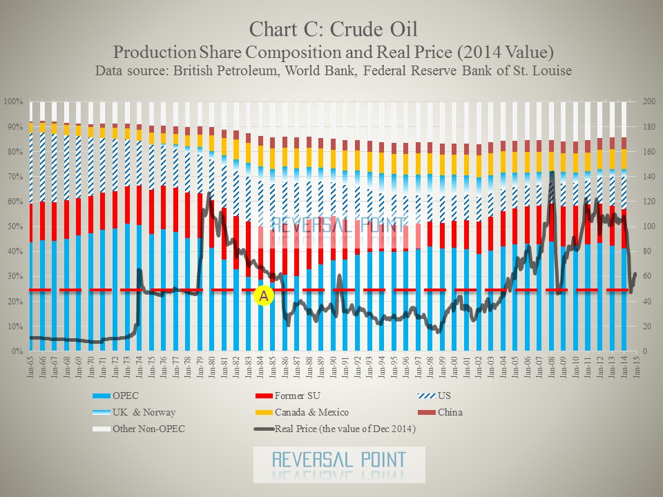
However, such a favourable negative correlation turned out to be short-lived. The decline in its production level had not defended the desirable price range because of production increases by non-cartel producers. The production share expansion among non-OPEC producers had become pronounced by 1985. In Chart C, the UK and Norway portions reflect their North Sea offshore expansion, while the Mexico portion represents some of the Gulf of Mexico oil production. As a result, in 1985 OPEC reversed its strategy in the name of its market share defence: the yellow circle mark with the letter A identifies this point of reversal in the chart.
The technical analysis may create some room for argument. Of course, technical analysis, since it is a popular guideline in trading culture, might induce a self-fulfilling prophecy to the extent that the market believes it. Behavioural finance might support this idea. According to Robert Schiller, market expectation plays a critical role in market price formation. Exposed to any new evolving context, however, the $50 demarcation line of the past could become obsolete or irrelevant in the new context and might not warrant the future ceiling of competitive market regime, or the future floor of the oligopoly regime to come. In order to draw the new demarcation line, we need to reflect the new underlying evolution. (To be fair, it should be noted that Mr. Kaletsky referred $50 as his assumption on shale oil players marginal cost, therefore, his argument is beyond a simple technical analysis.)
The technical analysis may create some room for argument. Of course, technical analysis, since it is a popular guideline in trading culture, might induce a self-fulfilling prophecy to the extent that the market believes it. Behavioural finance might support this idea. According to Robert Schiller, market expectation plays a critical role in market price formation. Exposed to any new evolving context, however, the $50 demarcation line of the past could become obsolete or irrelevant in the new context and might not warrant the future ceiling of competitive market regime, or the future floor of the oligopoly regime to come. In order to draw the new demarcation line, we need to reflect the new underlying evolution. (To be fair, it should be noted that Mr. Kaletsky referred $50 as his assumption on shale oil players marginal cost, therefore, his argument is beyond a simple technical analysis.)
Operating Decisions:
Temporary Suspension or Permanent Exit
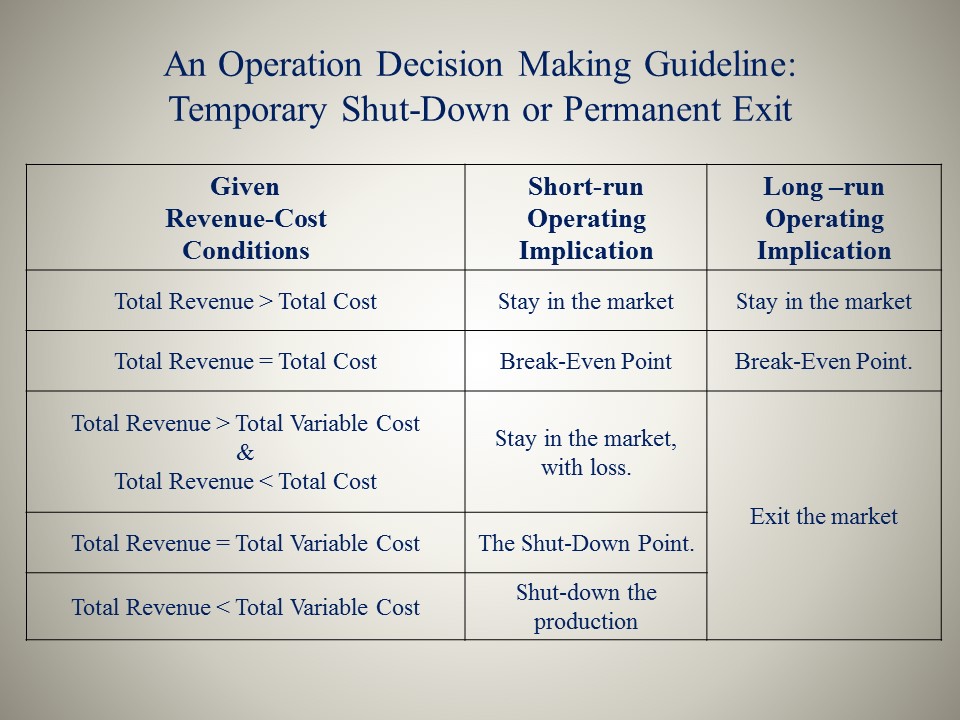
It should be fair to assume that the deterrence game would last until the top dog becomes convinced of either the victory or the defeat of its targeted competitors. To begin with, the top dog needs to be aware of the relationship between the price level and the decision-making process of the followers. At what price will the followers shut down their operation in the short-run and permanently exit in the long run? Without understanding the follower’s threshold, the top dog would fail to set the price target effectively for its Stackelberg game.
For reference, the box below outlines the general operation decision criteria between “short-term shut-down” and “long-run exit.” The following guideline is instructive: the relative level of the current price along the cost structure plays a key factor in determining the time horizon of the game.
For reference, the box below outlines the general operation decision criteria between “short-term shut-down” and “long-run exit.” The following guideline is instructive: the relative level of the current price along the cost structure plays a key factor in determining the time horizon of the game.
Evolution:
Technological Advancement by Game Changer
Jeffrey Currie provides another, evolutionary view. In late 2014, when many analysts were still expecting the crude oil price to recover to the previous level of $80-100, Currie surprised the market with his forecast that the crude oil price might plunge to $39. He set the floor level at $39, at which the bottom quartile high-yield E&P (exploitation and production) companies in the US would default (Surveillance/ Bloomberg TV, January 14, 2015).
The real surprise was the underlying transformation behind his floor price expectation. According to Currie’s analysis, the shale oil industry achieved a milestone technological advancement that transformed the E&P process from a conventional risky gambling-like process into a better-controlled manufacturing-like process. As a result, crude oil production in the shale oil industry has become more predictable and more flexible, and therefore, less risky (Currie, 2015, January 26). Below are highlights of Currie’s arguments.
The real surprise was the underlying transformation behind his floor price expectation. According to Currie’s analysis, the shale oil industry achieved a milestone technological advancement that transformed the E&P process from a conventional risky gambling-like process into a better-controlled manufacturing-like process. As a result, crude oil production in the shale oil industry has become more predictable and more flexible, and therefore, less risky (Currie, 2015, January 26). Below are highlights of Currie’s arguments.
- Supply: The control of the production volume has become easier than ever. Shale oil technology transformed E&P operations, making them less CAPEX intensive and more driven by variable costs. Lead time between capital injection and production start has collapsed from 4-5 years to roughly 28 days due to shale oil technology. This accelerated the speed of the production response to the mobilisation of capital. The shale oil production process transformed the supply curve, making it much flatter. This means that the price has become less sensitive to a given volume change, indicating better price stability.
- Market structure: As a consequence, OPEC, the oligopoly cartel, has abandoned pricing power. (Currie, December 15 2014) [2]
In other words, the innovation accelerated the speed of the production response to the mobilisation of capital. This suggests two important implications. One is for capital, the other for market expectations. In terms of capital, “the long-run asset value of shale oil reserves bodes well for their ability to attract capital, capital investments are now part of the adjustment process” (Courvalin, Currie, & Banerjee, May 2015). In terms of the market expectation, the market should quickly reflect the resulting supply response to a given change in price. A rise (decline) in price due to other factors, such as an increase (decrease) in demand, would give shale oil players a motive to mobilise (withdraw) the capital with the shortened lead time (about 28 days) to increase (decrease) production. Although the relative cost efficiency of shale remains inferior to that of Saudi Arabia, the positive transformation would give shale oil players a wider margin for survival.
Currie’s analysis advocates a case for innovation-driven deflation, therefore, good supply-driven deflation (click for "Demand-driven Deflation vs Supply-driven Deflation"). For further detail of his analysis, readers are encouraged to follow up his research related announcements on Goldman Sachs website.
Currie’s analysis advocates a case for innovation-driven deflation, therefore, good supply-driven deflation (click for "Demand-driven Deflation vs Supply-driven Deflation"). For further detail of his analysis, readers are encouraged to follow up his research related announcements on Goldman Sachs website.
Combined View: Supply-driven, Cost-deflation
Legacy's Survival v.s. Challenger's Innovation
The remarkable transformation of the shale oil industry could have been a surprise to Saudi et al of the oil cartel, OPEC, which allegedly imposed the deterrence game. Given this new information, an astute game leader now would return to the principle of Bayesian decision-making to reassess the viability of the deterrence game, by incorporating the new information into the assumptions of the deterrence game model. New conditions are likely to impose on the top dog either a longer time horizon or a much lower price level (or even both) to assure the better success of the deterrence game than initially anticipated. The deterrence game might be proven “not cost effective.” It may even turn out to be detrimental to both sides—the top dog and the followers—or to entire suppliers. It also may only benefit the demand side. A question is whether the top dog can stop or modify the game. If not, the original deterrence plan might result in a self-defeating game.
Furthermore, a new advancement in substitutes, such as solar panels, would add greater uncertainty to the pricing dynamics.
“Supply-driven deflation” emanating from structural transformations within the production space in primary resources would likely have a positive ripple effect for other sectors of the aggregate economy, especially those relying on these primary inputs, e.g., in manufacturing and construction, at least in the short to medium term, ignoring the effects of hedging transaction. The supply-driven cost deflation could improve their profit margin and its positive impact might penetrate greater areas of the economy. This might lead to a positive deflationary pressure, which would not harm economic growth.
Now, in order to simplify the argument, let us look at deflation impact in two categories along P/L within the financial statement context: revenue deflation and cost deflation. Cost deflation would have positive implications for corporate profitability, while revenue deflation would have negative ones. Of course, in reality the two can be compounded in a much more complex manner. We would need to reflect the dynamic interaction of the two factors to anticipate the net aggregate effect. Since deflation is a general term to represent decline in aggregate price, a separation into such a dichotomy has its limitations. Despite that, this conceptual distinction would give us some insight into the dynamics of the economy.
Repeatedly, during this period, there were other important developments that affected the supply-demand imbalance. Since this chapter has focused mainly on the mechanism behind the astounding magnitude of price decline in crude oil, it has highlighted only the relevant and critical factors discussed above and left out the others. In order to gain a more comprehensive view beyond the focus of this discourse, readers are encouraged to refer to other sources regarding other developments within the crude oil sector during this period, such as softening demand and geopolitical factors.
Notes:
1. Kaletsky uses the term “monopoly” throughout his exposition. In order to better reflect the actual market structure of crude oil industry, his use of the term “monopoly” is replaced with “oligopoly” throughout this writing.
2. . Besides those supply factors, Currie also addressed demand factors: the US has become self-sufficient and a base-load demand for crude oil, therefore, is no longer a marginal consumer; now the marginal demand comes from emerging markets (Currie, December 15 2014). Since this chapter has a focus on supply side dynamics, it will not cover demand factors in detail.
Copyright © 2015 by Michio Suginoo. All rights reserved.
Reference
- Bloomberg. (n.d.). Market Quote of WTI Crude Oil (Nymex). http://www.bloomberg.com/
- Chevalier-Roignant, B., & Trigeorgis, L. (2011). Competitive Strategy: Options and Games. Cambridge, Massachusetts: The MIT Press.
- Courvalin, D., Currie, J., & Banerjee, A. (2015, May). The new oil order: a self-defeating rally. Commodity Research, Goldman Sachs. Retrieved from: http://www.goldmansachs.com/
- Currie, J. (2014, December 15). The new oil order. Exchanges at Goldman Sachs. Video retrieved from: http://www.goldmansachs.com/
- Currie, J. (2014, December 15). The new oil order. Exchanges at Goldman Sachs. Podcast retrieved from: http://www.goldmansachs.com/
- Currie, J. (2015, January 26). So, what is the “New Oil Order”? Top of Mind. Issue 31. p4.
- Kaletsky, A. (2015, January 14). A new ceiling for oil prices. Project Syndicate. Retrieved from: http://www.project-syndicate.org/
- Piros, C. D., & Pinto, J. E. (2013). Economics for investment decision makers. Hoboken, New Jersey: John Wiley and Sons, Inc.
- Reserve Bank of Australia. (2015, February). Box A, the effects of changes in iron ore prices. Statement of Monetary Policy. Reserve Bank of Australia. Retrieved from: http://www.rba.gov.au/
- Surveillance/Bloomberg TV. (2015, January 14). Shale fundamentally changed oil market: Goldman's Currie, Bloomberg TV, Video clip retrieved from: http://www.bloomberg.com/
- Surveillance/Bloomberg TV. (2015, February 20). Oil can drop to $39 a barrel: Goldman Sachs Currie. Video clip retrieved from: http://www.bloomberg.com/