REVERSAL POINT
  • Home
    • Your Support
    • Privacy Policy
    • Terms of Use
    • Contact
  • Monetary Paradox
    • Monetary Wonderland
    • Shirakawa's Monetary Policy Paradox 1
    • Shirakawa's Monetary Policy Paradox 2
    • Minsky's Non-Neutral Money
    • Monetary Policy Paradox
  • Secular Cycle
    • Blog >
      • Bond Wave >
        • Monetary Regime Cycle and BitCoin
        • Paradigm Shifts in Monetary Regime along Bond Wave
    • Supra-secular rhythm
    • Secular Rhythm of Bond Wave >
      • Bond Wave Mapping 1: Paradigm Transformation in Interntional Monetary Regime
      • Bond Wave Mapping 2: Price & Inflation Cycles
      • Bond Wave Mapping 3: Private Debt Cycle
      • Bond Wave Mapping 4: Fiscal Cycle & Negative Real Yield Cycle
      • Bond Wave Mapping X: Political Cycle
      • Limited Gold Supply was a perennial problem for the Gold Standard: in search for Elastic Money and Scalability
  • Political Philosophy
    • Zeitgeist Zero Hour: Intro
    • Socrates Constitutional Cycle >
      • Socrates' Constitutional Cycle
      • Intrinsic value of Socrates Cycle
      • Contrast between Socrates vs Aristotle
    • Can we preserve democracy? >
      • Terminal Symptom of Democracy in Ancient World, Theoretical Views
      • Paradox of Equality & Aristotelean Paradox Management
      • Aristotelean Preservation of Constitutions
      • Contemporary Liberal Representative Democracy?
    • Old Contents >
      • Socrates' 5 Political Regimes
      • Socrates-Homer Hypothesis
      • Crassus & Trump: Socrates-Homer Hypothesis in Modern Context
  • Others
    • Price Evolution >
      • Oligopoly Price Cycle
      • Deflation >
        • Zero Boundary
        • Anecdote 1874-97
        • Deflationary Innovation
    • Innovation >
      • Introduction AI & ML & DL >
        • Chap1 ML Paradigm
        • Chap2 Generalization of ML
        • Chap3 DL Connectionism
        • Chap4 DL Learning Mechanism: Optimization Paradigm
        • Chap5 DL Revolution
        • Chap6 DL Carbon Footprint
        • Chap7 DL Underspecification
        • Chap8 CNN & Sequence Models
      • Map Risk Clusters of Neighbourhoods in the time of Pandemic
      • Confusing Blockchain >
        • Chapter 1: Linguistic Ambiguity
        • Chapter 2: Limitations in Consensus Protocols
        • Chapter 3-1: Disintermedition Myth-conceptions
        • Chapter 3-2: Autonomous Self-regulating Governance Myth-Conceptions
    • Environmental Distress >
      • Model Risk and Tail Risk of Climate-related Risks
  • Socrates' Constitutional Cycle

Series:
Basic Intuitions of Machine Learning & Deep Learning for beginners


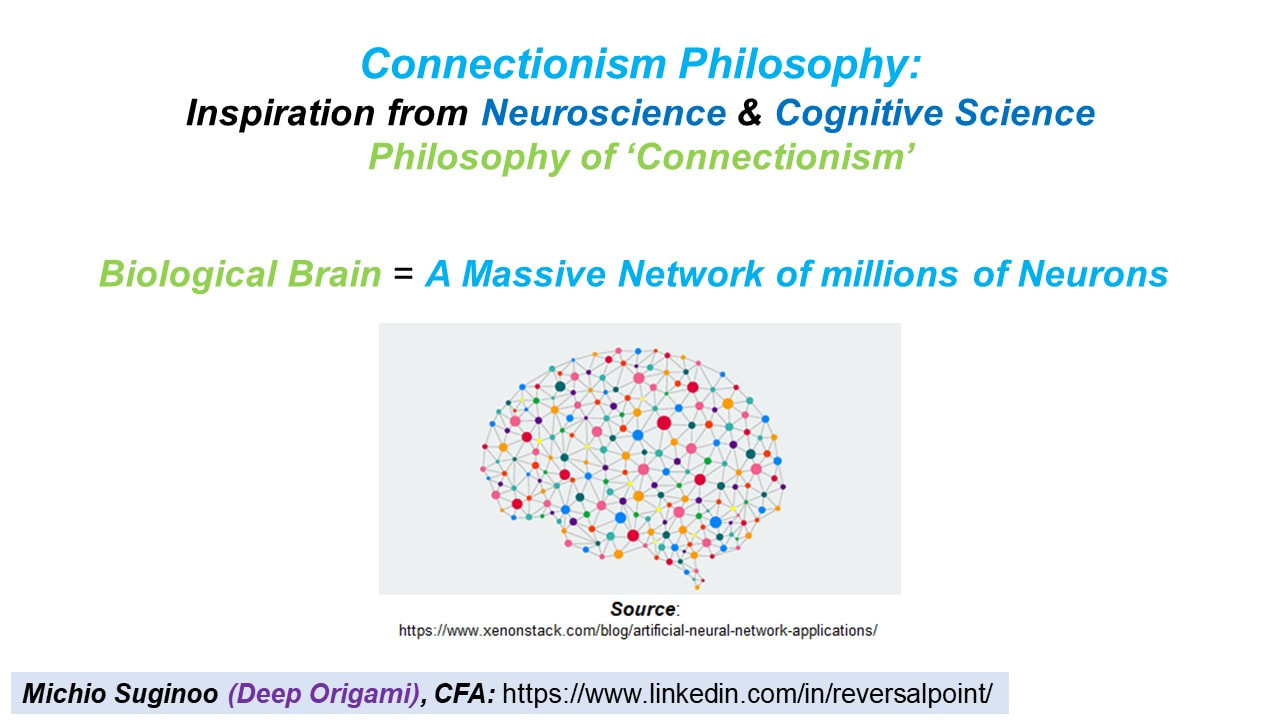
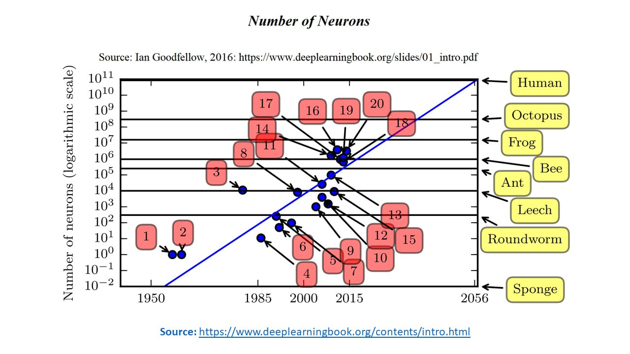
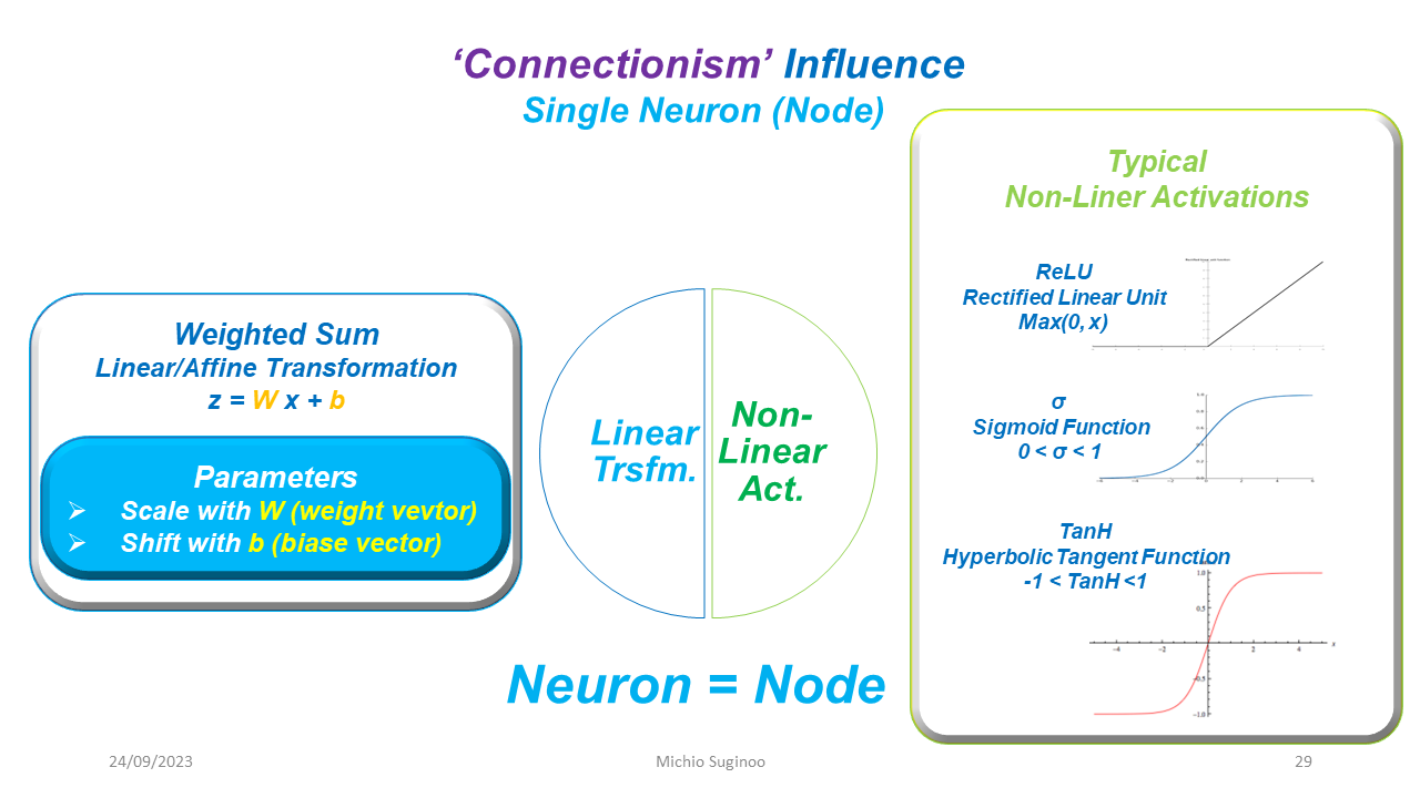
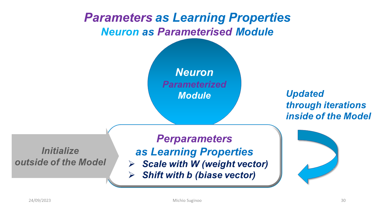
Chapter 3: Deep Learning Connectionism Architecture
Philosophy of Connectionism

Originally published 16 February, 2021
By Michio Suginoo

Picture
The architecture of Deep Learning is inspired by Neuro Science and Cognitive Science, and particularly by the philosophy of Connectionism.

A biological brain is a massive network of many neurons.

The chart below compares the number of neurons among different types of creatures. And Human ranks on the top after Octopus. (Goodfellow, Bengio, & Courvil, 2016, p. 23)
Picture
And Connectionism speculates that:

While each single neuron can only execute simple operations as an individual unit, when many neurons are connected together as a massive neural network, they can collectively exhibit very intelligent behaviours.

Deep Learning incorporates this notion into its architecture.

Simplicity of a single Neuron (Node)

Now, in the next figure, I want to show you how simple a single neuron can be. The circle in the middle represents one single neuron, which is also called a Node. It is the fundamental building block of Deep Learning.
Picture
It does only two simple operations: first it receives an input from the previous neuron and executes a linear transformation on the input (on the left in the chart) and passes the result to non-linear activation (on the right in the chart). And ultimately, it passes the result of the activation to the next neuron(s).

Linear Transformation (Affine Transformation)

The linear transformation applies to the input two vectors—namely, weight and bias. They only scale and shift the input: no more, no less. Nevertheless, they play an essential role in storing and updating learning properties. They are called hyperparameters, which is explained shortly.

Here is a couple of paragraphs for a little deeper understanding about the linear transformation, if you like: the linear transformation is an affine transformation. It does not change certain characteristics among the input components such as ratio of distances and alignment of certain points.

Affine Transformation:
“An affine transformation is any transformation that preserves collinearity (i.e., all points lying on a line initially still lie on a line after transformation) and ratios of distances (e.g., the midpoint of a line segment remains the midpoint after transformation). In this sense, affine indicates a special class of projective transformations that do not move any objects from the affine space R^3 to the plane at infinity or conversely. An affine transformation is also called an affinity.”
So, an affine transformation preserves:
  1. collinearity (i.e., all points lying on a line initially still lie on a line after transformation) and
  2. ratios of distances (e.g., the midpoint of a line segment remains the midpoint after transformation)

If this additional info about the linear transformation (Affine Transformation) does not appeal well to your intuition, do not worry. You can skip this part. This was just an extra insight. For now, in order to cultivate your intuitions, you can move forward skipping it.

Non-linear Activation


Now in the box on the right, we have the graphical representations of three typical non-linear activations. As you see, each of these charts represents an execution of a very simple non-linear operation.

Here are some intuitions about these three activation functions:
  1. ReLU (Rectified Linear Unit): At the beginning, it was hard for me to believe that ReLU is one of the most popular activation functions used in the hidden layers for two reasons: it’s almost linear; it’s debatable whether it is differentiable at the kinked point. Nevertheless, the notion of ReLU is inspired by the behaviour of biological neurons. Neuro Scientists discovered that a single neuron does only respond to signals with a certain minimum criteria of input value. Well, the criteria must be discovered in the linear transformation. In the activation, it only reacts to the positive result of the linear transformation.
  2. Sigmoid Function: Sigmoid outputs a probability proxy, taking any real value as its input to map it over the range between 0 and 1. So, it is used when we expect the output to have a probability proxy representation.
  3. TanH Function (Hyperbolic Tangent Function): TanH takes any real value and map it over the range between the negative 1 and the positive 1. When we have different types of inputs with different scales, it standardizes/normalizes the scale of the input.

Overall, a single neuron (node) executes only simplistic operations; thus, it is far from an intelligent entity.

Now, regarding a single neuron, I would like to make one more remark: it’s about Hyperparameter.

Hyperparameter

A Hyperparameter is a special type of parameter that needs to be initialized outside of the model.

Once initialized, they are continuously updated through iterations in the model.
Picture
Since hyperparameters are embedded within the architecture of neuron, a neuron is often called a “parameterized module”. And often a random value is assigned to its initial value.

That’s enough about a single neuron for now. Next, let’s take a look at “the neural networks as a whole”. Remember, Connectionism speculates: while a single neuron executes only simple operations, when multiple neurons are connected, they collectively exhibit an intelligent behaviour as a neural network.

What makes Neural Network as an Intelligent Entity?

What you see in the next figure is a morphology of Deep Learning Algorithm in the form of Computation Graph. Computation Graph is a graphical representation of computation. The most important take away in this slide is: Deep Learning operates two kinds of computing: Parallel Computing and Sequential Computing.
Picture
On the left, we have one single layer containing multiple neurons. Within one single layer, multiple neurons behave together without any connection. So, a layer represents a parallel computing, which demands intensive real time processing. A layer constitutes a building block of Deep Learning.

On the right, we have a stack of layers. The name, Deep Learning, is derived from this particular morphology of the stack of layers in its architecture. And connections run from one layer to the next through neurons in sequence. The stack of layers represents Sequential Computing.

Overall, Deep learning, while processing information in parallel, learns in sequence.

As a precaution, this illustration represents one of the most basic prototype of Deep Learning model called ‘Feedforward Neural Networks’. Usually, viable Deep Learning models have far more complex structure. As new models sought for a better performance, the layers of their architecture deepened. The next historical chart reveals this notion.
Picture
This is the historical evolution of the depth of layers in the top competing models in a prominent computer vision contest, Large Scale Visual Recognition Challenge, a.k.a. ILSCRC.

You see the # of layers on the top of the bar charts.

Deep Learning was introduced to this contest with the model called AlexNet in 2012. Until then, the # of layers used to be 1.

Nevertheless, AlexNet was not the first Deep Learning model. In the 1960s, the earliest generation of Deep Learning was introduced. Nevertheless, it failed to perform well, because it could not extend its layers enough due to the hardware constraint at that time. This paints a symbolic picture: the evolution of Deep Learning is significantly influenced by the evolution of hardware.

All that said, it turns out to be: simply adding layers does not necessarily improve the performance. It is because often a deeper model is difficult to optimize.
Simply put, to determine a right depth of layers is a tricky business, and would require engineering expertise.

Complexity and Simplicity of Deep Learning


In a nutshell, Deep Learning is a complex network of simple neurons. Complexity and simplicity are both coexisting in the architecture of Deep Learning.
Picture
And its complexity can be captured by the size of “its 4 operating components”:
  • # of neurons or nodes
  • # of hyperparameters
  • # of layers
  • # of connections.
Today, the complexity of Deep Learning Models is exploding.
 
In Chapter 5, we will see some implications of the exploding complexity of Deep Learning today.

In this chapter, we saw the simplicity and the complexity of the neural network architecture of Deep Learning. In the next chapter, let’s find out the learning mechanism of Deep Learning. How does it learn?

Donation:
Please feel free to click the bottom below to donate and support
the activities of www.reversalpoint.com

​Copyright © by Michio Suginoo. All rights reserved.

Proudly powered by Weebly