Bond Wave Mapping 3: Private Debt Cycle

BOND WAVE MAPPING: CASE STUDY 3
Private Debt Cycle Along the Bond Wave

Originally published July 23, 2016
Last edited January 2, 2022
by Michio Suginoo

This section reviews the private debt cycle along the bond wave.

A detailed definition of the bond wave is described in Secular Rhythm of Bond Wave.

Sidney Homer left us a notion that the state of money has something to do with the evolution of the Western civilization. And it extends to a scale of one life cycle of civilization. In studying the bond wave, I intend to apply Homer’s notion in a shorter horizon, say secular time frame. In other word, we can use the bond wave to observe a long-term transformation in the relationship between bond yields and other metrics. My attempt is to capture a notion that the state of money mirrors a broader socio, political, and economic reality.

Bond wave mapping provides a heuristic approach to apply historical analogy to make relevant questions about our present and future based on our past.

Overview: Secular Rhythm of Private Debt-Money

The Global Financial Crisis of 2007/8, emanating from the collapse of the subprime loan bubble in the United States, became an international financial contagion across boarder. And it took place during the most recent bull bond cycle, or the Globalization Wave (the 1980s-today as of 2020) in the Bond Wave term.

The development of the debt-fueled financial crisis in the United States can be viewed in a cyclical framework that is comprised of the following chain of events:

Economic stability, accompanied by low interest rates, drove debt-fueled excess demand;
the excess demand translated into an economy of scarcity, or supply shortage, and raised price and profit margin;
a higher profit margin legitimized an expansion of supply capacity;
when the bubble busted, deleveraging process kicked in and it gave rise to deflationary pressure;
sales price fell and profit margin was squeezed;
the supply expansion that had been embarked during economic stability completed with a time lag, resulting in an economy of excess/abundance;
the abundance/excess in supply capacity amplified the deflationary effect that deleveraging process triggered and further reduced the profitability;
deflation drove down the cost of innovations: cost-cutting innovations were deployed in production process to reduce labour costs;
reduction in profitability compelled business to cut down the fixed costs and introduce new innovation into production;
it changed the market structure of job, reducing labour demand.

Of course, besides these events, this period was accompanied with other trends—e.g. hollow-out, outsourcing of manufacturing functions to developing economies—amplifying the structural shift of economy.

In this chain of events, the role of money was significant. Changes in money supply transformed the structure of real economy. In other words, this period manifested the non-neutrality of money that Hyman Minsky articulated. This reading reviews the non-neutrality of money through private debt cycle along the bond wave.

In hindsight, a similar, if not the same, chain of events--the Wall Street Crash of 1929 and the Central European Banking Crisis of 1931--took place during the previous bull bond cycle, which corresponds to the Vacuum Wave (1920-1945) in terms of the Bond Wave.

In other words, both of these two bull bond cycles manifested "private debt cycles": debt-fueled bubble economy and its ensuing destructive systemic financial crises.

Briefly, the two bull bond cycles--the Vacuum Wave and the Globalization Wave--demonstrated two similarities below.

Each bull wave contained one private debt cycle, which is measured by the private debt to GDP ratio.
Each bull wave experienced a persistent decline in the real velocity of money after the systemic financial crisis.

In this section, we project the secular rhythm of private debt activities over the bond wave. More specifically, we apply “bond wave mapping” over four metrics below:

Private debt level;
Private debt to GDP ratio;
Velocity of money; and
Money multiplier.

As a reminder, the five bond waves are defined as follows:

the Victorian Wave from 1798 to 1897;
the International Gold Standard Wave from 1897 to 1920;
the Vacuum Wave from 1920 to 1946;
the Reconstruction Wave from 1946 to 1981; and
the Globalization Wave, ongoing since 1981.

These systemic financial crises distinguish themselves from other types of economic distress in the following aspects.

International Contagion (epicenter and transmission hub): These two crises spread across advanced economies and peripheries through the international financial centres, namely London and New York. In the Global Financial Crisis (2007/8), the negative impact of the US subprime mortgage crisis spread rapidly worldwide. As a background, the risks of the US sub-prime loans were packaged in securitized products and sold across major economies. When the collapse in the subprime loans in the United States triggered a financial contagion across boarder like a wildfire. In comparison, the Great Depression unfolded through two steps: first, the Wall Street Crash in 1929 was “largely a U.S. phenomenon”; second, the Central European Banking Crisis of 1931, emanating from central Europe, was transmitted via London to become “a worldwide contagion.” On one hand, it could be deemed that the link between the American stock market collapse of 1929 and the global contagion of the systemic banking crisis of 1931 is tenuous in the Great Depression; on the other, the fact that capitals that had moved to the central Europe from the United States during the 1920s actually reversed in the 1930s suggests a link between the two incidences. (James, 2009) Nevertheless, despite differences, both the Vacuum Wave and the Globalization Wave share these two notions: core financial centres of global economies, namely London and New York, acted as transmission hubs to make these crises as financial contagions; and banking systems played a core role to unfold systemic financial crises.
Deflationary Pressure (Reduced Velocity of Money, Compression og Net Asset): These two crises were preceded by extraordinary leveraging processes. They were products of debt deflation. Although these two crises demonstrated different magnitudes of economic distresses, they also demonstrated some common features. As Irving Fisher illustrated, debt deflation caused reduced the velocity of money and compressed net assets in the system.
The scale of government interventions: although the measures taken differ between these two cases, massive government interventions ensued: fiscal expansion for the former case; monetary expansion for the latter.

The creation, destruction, and evaporation of modern money

Modern money is primarily created (or destroyed) through two major dynamics: debt creation (repayment) through commercial lending in the private sector; and monetary policy adopted by central banks (McLeay, Radia, & Ryland, 2014, p. 16).

Commercial lending is a private sector’s money creation activity: debt money increases by lending and decreases by repayment, and even evaporates through defaults in the system. More importantly, money is not neutral, since it affects real economy in the long term.

According to Hyman P. Minsky (1985), the state of economy shapes the psychologies of economic actors—savers, lenders, and borrowers. Changes in the state of economy can transform their profit expectations (income expectation and expenditure preferences) and liquidity preferences and, ultimately, more diversely their economic behaviours. Then, changes in their behaviours feed back into the state of economy. The period of economic stability bring optimism in the psychologies of these economic actors and induce them to expand the leverage in the system:

savers spend more than they save;
lenders seek an expansion of their market share in lending; and
borrowers justify their borrowing for profit (or utility) expansion.

Then, it transforms the state of economy from stability to instability in the following order:

the net debt level increases and the debt money expands;
as time goes by, the increase in financial leverage becomes excessive: excess debts account for a destabilising factor;
when the momentum of the economic stability recedes, the excess leverage in the system results in a series of default in debt-service;
as a consequence, debt money evaporates. (Minsky, 1992, pp. 7-8; 1985, p 13)

Consequential deleveraging becomes destructive to the economic system. If it involves corporate sector, it would compel business to mobilise new innovations to cut labour cost. A dire job expectation destroys consumptions, consequentially, the aggregate demand. It would annihilate the money multiplier in the long run. As Hyman Minsky noted, “stability is destabilising,” and money affects real economic activities: therefore, money is non-neutral. And real economy goes on from one state of disequilibrium to another and ultimately fails to revert to its equilibrium, proving that economic forecasts based on equilibrium are nothing but fallacy.

Private debt cycle metrics

To capture the rhythm of the private sector’s debt money (i.e., expansion, destruction, and evaporation) along the bond wave, this readings applies bond wave mapping on the following metrics:

the private sector’s debt level, both in dollar terms and in relative terms in relation to GDP to gauge leverage in the system;
the velocity of money to gauge debt money’s non-neutral impact on the economy; and
the money multiplier to gauge the effectiveness of the monetary base in promoting the creation of the private sector’s debt money and its circulation.

Due to constraints in the availability of statistics, we trace both the US private debt level and velocity of money only after 1916.

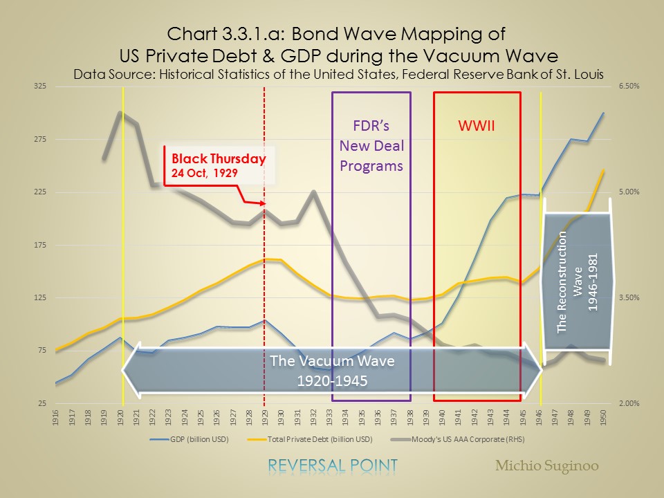
Private Debt Cycle during the Vacuum Wave

The following three charts—Chart 3.3.1.a, Chart 3.3.1.b, and Chart 3.3.1.c—cover the period 1916 to 1950 to illustrate the evolution of US private debts around the Great Depression. While the first chart measures the level of private debts and GDP in dollar terms, the second chart traces the relative ratio of private debt to GDP. The third gauges the money multiplier, the driver of credit money creation in the private sector.

In Chart 3.3.1.a:

The debt level rises from $76.5 billion at the beginning of the chart;
It more than doubles at its peak in 1929, the year of Black Thursday, reaching $161.1 billion;
Thereafter, it reverses the course, together with GDP, to demonstrate the post-crisis deleveraging process by dropping by about 22% toward the Presidency inauguration of Franklin D. Roosevelt (FDR) in 1933; and
Finally, with a series of massive fiscal expansions throughout the New Deal Program era, it stabilizes within a reasonably narrow range until the beginning of the WWII.

During the war, the debt level rises moderately, by 17% from its pre-war bottom to $144.7 billion at the end of the WWII; entering the period of the Reconstruction Wave, its post-war level restores upward momentum, together with GDP, to significantly exceed the pre-crisis level.

Total Private Debt to GDP Ratio

Now we shift our attention to the private debt in relative terms. In Chart 3.3.1.b, "the total private debt-to-GDP ratio" captures one debt cycle along the bull bond market of the Vacuum Wave (the 1920s-1945). The metric measures the proportion of leverage in the system relative to GDP.

In 1920, at the start of the bull bond market, it starts expanding from a level around 122% . And it peaks at 233% around the middle of the bull bond market in 1933. Thereafter, it bottoms at 63% in 1945 at the end of the bull bond cycle. This timeline demonstrates a remarkable synchronization between the private debt-to-GDP ratio and the Vacuum Wave. Caution is needed for this interpretation. This notion of synchronization is no more than a synchronization that one private debt cycle (a pair of rising and declining waves) fits into one single bull wave.

The peak in the debt-to-GDP ratio lags that of the debt level. During this lag, the ratio continues to increase, it is because the denominator, GDP, declines more drastically than the numerator, debt level, during the period between Black Thursday (1929) and the introduction of the New Deal program (1933). Therefore, the surge in the debt-to-GDP ratio’s (in the absence of a rise in debt level) is a manifestation of the destructive impact of the Great Depression on GDP, economic growth. This destruction is expressed in the rapid decline in the velocity of money in the same chart.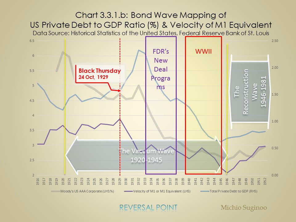

How money affects GDP

Velocity of Money

Now, we briefly overview the manifestation of non-neutrality of money—in other words, how money affected GDP—by tracing the velocity of money: GDP divided by M1 or M1 Equivalent. Although the velocity of money might not be considered as a measurement of non-neutrality of money, it illustrates the impact of money on GDP in its trajectory.

M1 is a measurement of money in circulation. Since the Federal Reserve Bank did not release M1 statistics before 1959, for the period prior to 1959 we must employ a proxy for M1 to construct the chart approximating the velocity of M1 money stock: Friedman & Schwartz’s M1 series before 1946; Rasche’s M1 series for 1947 to 1958. (Carter et al., 2006, pp. Vol 3: 604-607) We call these proxies collectively “M1 Equivalent” for our discussion purposes. We measure the velocity by dividing GDP by M1 Equivalent. Chart 3.3.1.b illustrates the trajectory of the velocity of M1 Equivalent from 1916 to 1952.

The velocity measure, after increasing from 3.04 to 3.67 during the period 1916 to 1920, remains high, with the exception of a dip from 1921 to 1922, peaking at 3.89 in 1929, the year of the Wall Street Crash. Thereafter, it reverses direction downward to the end of WWII, although it demonstrates some stability during the New Deal era and some rebound in the mid–WWII period. In brief, until the beginning of the succeeding bear bond cycle, the Reconstruction Wave (1946-1981), the velocity of money fails to demonstrate a sustainable recovery.

In principle, the velocity of money collapses significantly throughout the post-crisis period—from the Wall Street Crash in 1929 until the end of WWII (1945). This illustrates how the post-crisis deleveraging process diminished the velocity of money. Overall, the large-scale fiscal expansion of the New Deal and the WWII special war demand did not reverse the post-crisis collapse in the velocity of money. It took another massive fiscal expansion, the post-war reconstruction effort, to restore the velocity of money: it required a series of unconventional fiscal expansions and possibly the destruction of war. Here as well, the rhythm in non-neutrality of money and the bond wave demonstrate a remarkable synchronization.

Money Multiplier

Finally, Chart 3.3.1.c demonstrates “bond wave mapping” over the historical chart of money multiplier. The M1 money multiplier—M1 or M1 equivalent divided by the money base—gauges the transmission effectiveness of monetary base into money supply. Thus, it measures the private sector’s ability to create credit money.

Although monetary authorities can closely influence the monetary base, they can only loosely induce money multiplier to modulate money supply. Money multiplier measures the private sector’s ability to create credit money through commercial lending: this mechanism drives the circulation of money in the private sector.

As a matter of fact, this chart illustrates how indirect and uncertain monetary authority’s influence over the circulation of money could be.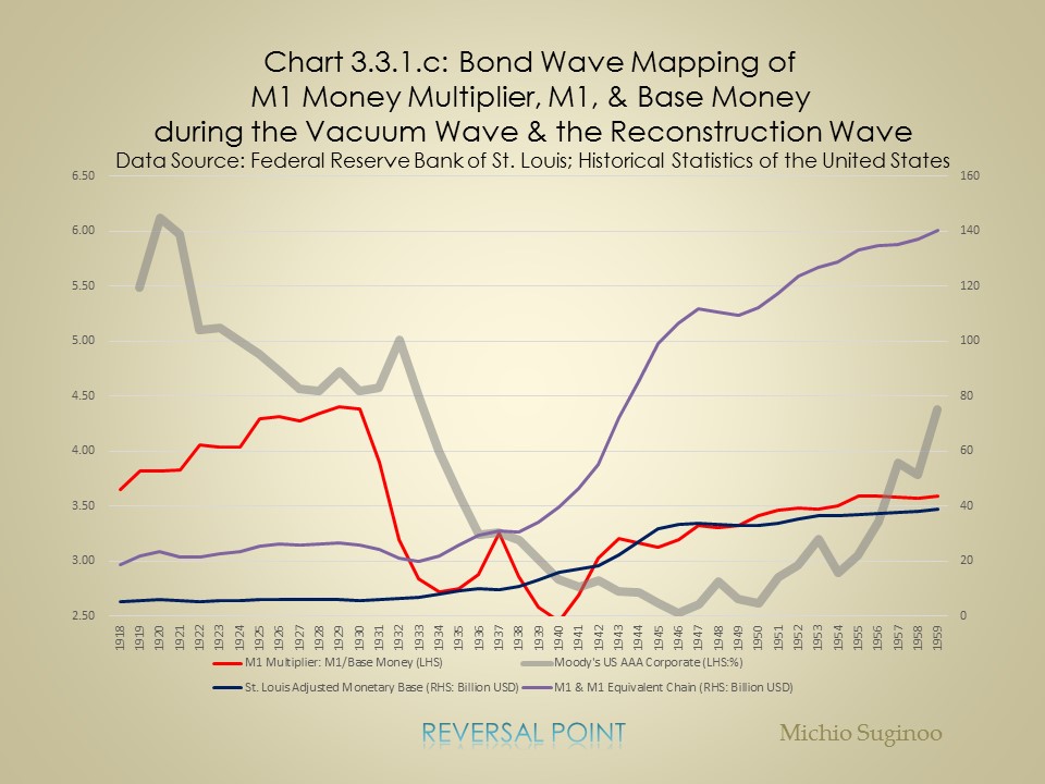

In 1929, the year of the Wall Street Crash, the money multiplier (M1 multiplier in the chart) reached its high at 4.4, then continued to remain relatively stable for one year, thereafter plunged toward 2.72 until1934. Along with the progression of the New Deal program, it made a transient recovery until 1937 to 3.25, then collapsed again until the year before the US participation in WWII. This suggests that, while the New Deal boosted the money multiplier for a short term, it was only transient and did not fully restore its sustainable mechanism. It took WWII—another massive fiscal expansion and the destruction of war—for the money multiplier to restore itself.

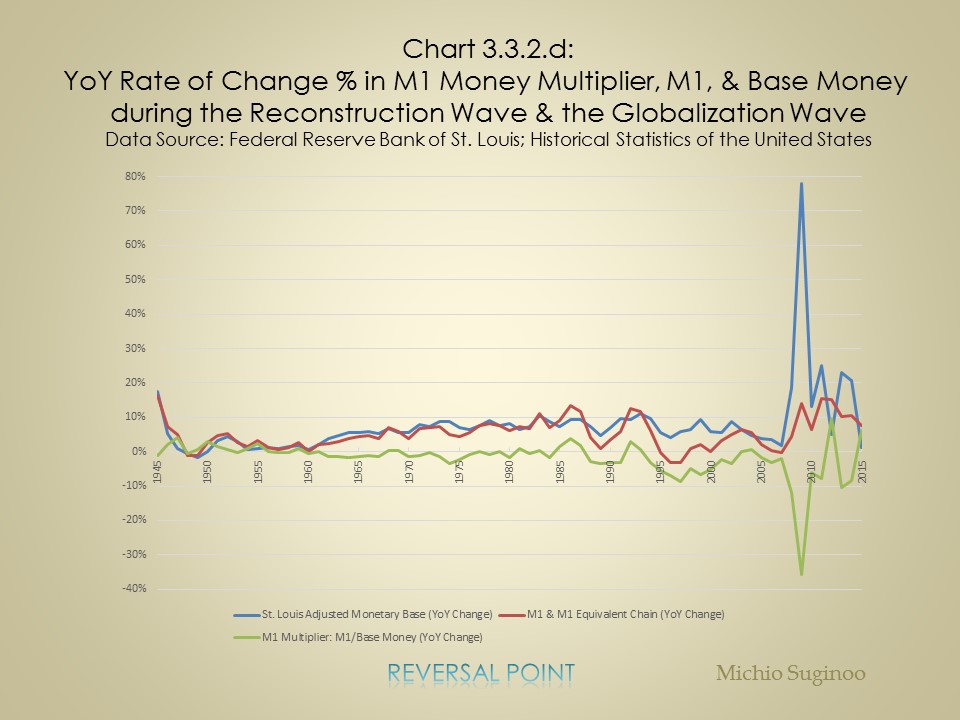
Now, in order to take a closer look at the interaction between the monetary base and M1 equivalent (money supply), Chart 3.3.1.d tracks year-over-year (YoY) change in both monetary base and M1. Overall, this chart reveals that the change in M1 equivalent (money supply) tends to lag the change in the monetary base. It is quite intuitive.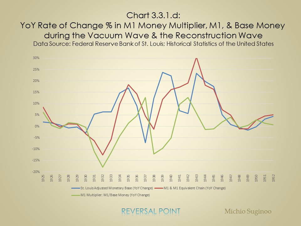

The one-year stability observed earlier in the money multiplier from 1929 to 1930 is because both metrics, M1 and the money base, declined moderately at comparable rates. Then, despite an increase in the YoY rate of change in monetary base up to 6% from 1930 to 1932, the YoY change in M1 made a remarkable decline. It required an even stronger rate of increase in the monetary base—from 6.4% to 18.4% from 1933 to 1935 to boost the YoY change in M1 money. The recovery in money supply (M1 equivalent) coincided with the early stage of FDR’s administration and the introduction of the New Deal programs (fiscal expansion).

Thereafter, for the rest of the New Deal era, the YoY rate of change in the monetary base again plunged from its peak of 18.4% in 1935 to –7.2% in 1937. Accordingly, M1 demonstrated a drop in its YoY rate of change. This implies that the absence of an increase in the monetary base might be associated with the plunge in M1 in the aftermath of the financial crisis.

Then, WWII reversed the course of events. From its onset, the YoY rate of change in M1 increased to 30.5% in 1943, lagging behind the drastic increase in monetary base that has taken place since 1938. Thereafter, despite a drop in its level, the YoY rate of change in M1 remains above the zero line, with a minor breach from 1948 to 49. This illustrates the background behind the remarkable recovery in the money multiplier after 1940.

So far, we have observed one historical debt-cycle case within a bond bull cycle of the Vacuum Wave (1920-1945). Next, we move to another case in the Globalization Wave (the 1980s-today as of 2020).

Private Debt Cycle
During the Reconstruction and Globalization Waves

Chart 3.3.2.a tracks the level of private non-financial debt and GDP during two bond waves—the Reconstruction Wave (1946-1980) and the Globalization Wave (1981-today as of 2020). The private non-financial debt level and GDP rose gradually at roughly the same rates during the Reconstruction Wave (1946-1980). Entering the Globalization Wave (1981-today as of 2020), the private non-financial debt level accelerated faster than the GDP and made its near-term peak at USD 24,741 billion in 2008 at the onset of the Global Financial Crisis. However, in contrast to the case of the Great Depression, it did not collapse afterwards. Instead, after a temporary setback, it kept rising. From this dollar term chart, the debt level does not form one cycle—a series of a rising and an ensuing declining trends—in contrast to the case of the Great Depression.

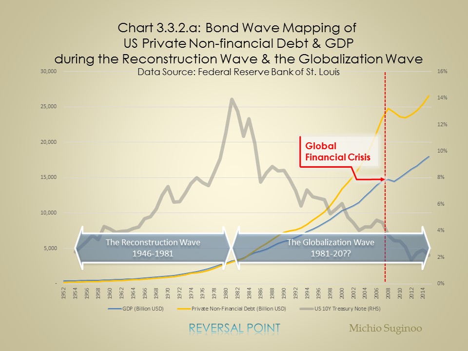
Chart 3.3.2.b measures US private non-financial debts in relative to GDP, showing its debt to GDP ratio. The ratio demonstrates a declining trend during the aftermath of the Global Financial Crisis (Chart 3.3.2.b). In 2008, the ratio peaked at 1.68, then declined notably for some time toward 1.46 until 2014 before stabilizing briefly.

Now when we trace the velocity of money, the impact of money on GDP, the presence of one cycle appear more clearly. In terms of the velocity of M1, it peaked at the outset of the crisis and collapsed toward the end of the Vacuum Wave. The velocity of money demonstrates analogy with the Great Depression case.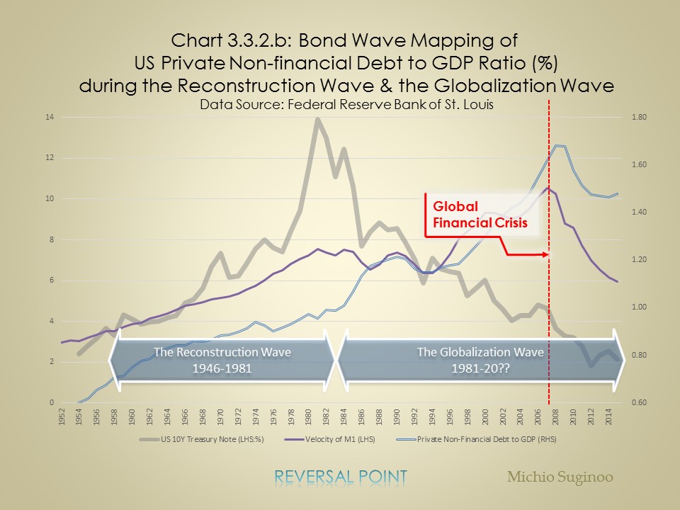

Now we turn to the money multiplier for this period in Chart 3.3.2.c. Like the previous case of the Great Depression, the money multiplier plunged rapidly after the outbreak of the Global Financial Crisis in 2007. Its level collapsed from 1.61 in 2007 to the historical low of 0.71 in 2014.

Nevertheless, a salient contrast can be seen in the trajectories of monetary base between the Great Depression and the Global Financial Crisis (dark blue lines in Chart 3.3.1.c and Chart 3.3.2.c, respectively). In the former case, the monetary base did decline in the aftermath of the crisis; in the latter case, it made a historic surge thanks to unprecedent quantitative easing (QE). Despite the historic boost in monetary base by monetary authority, money multiplier collapsed. This shows us that the increase in the monetary base was not effective in restoring the private sector’s ability to drive the circulation of money.

It also suggests that the historic expansion in liquidity supported the persistence in the level of private non-financial debt after the crisis (Chart 3.3.3.a). A natural ensuing process of deleveraging, an automatic adjustment mechanism to liquidate excess leverage in the aftermath of the systemic financial bubble, might have been paralyzed by the liquidity expansion. On the other hand, it failed to boost money multiplier. This suggests the lack of demand. This is a reflection of policy failures in restoring a primary driver of economy, income expectation and employment. This implies the need for a demand side measure.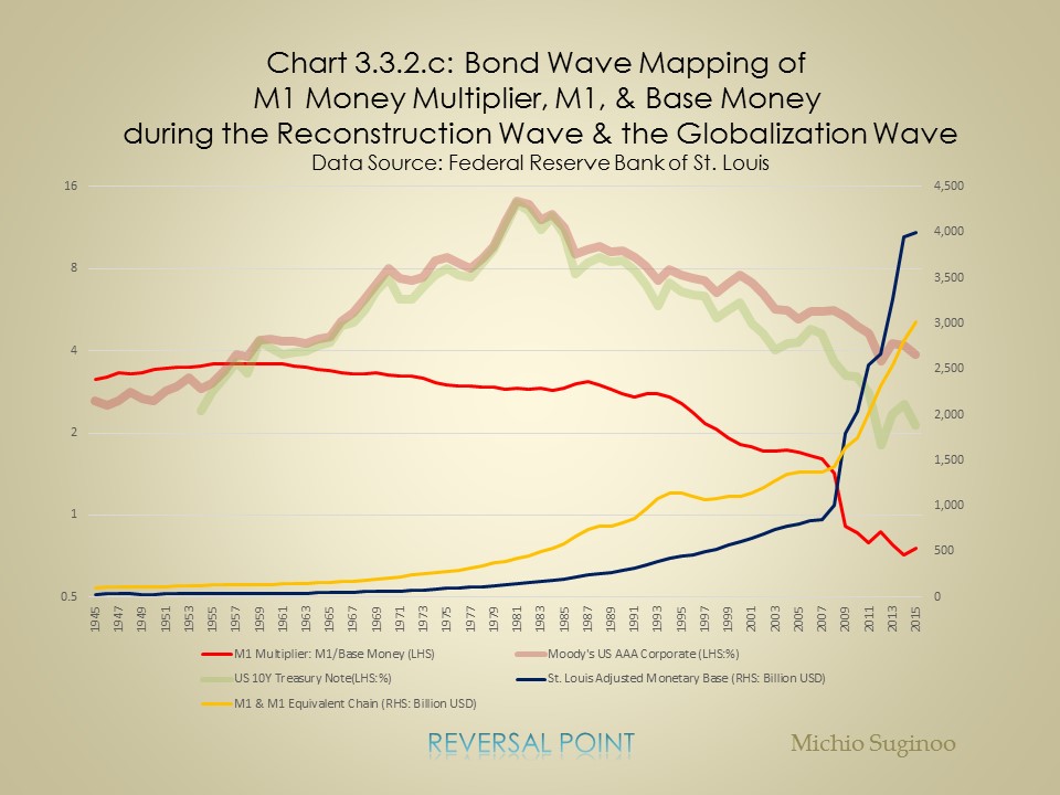

Since quantitative easing (QE) allowed the monetary authority to purchase private securities directly, the QE process does not necessarily involve an adjustment of monetary base in its passage. The monetary authority, through its direct purchase in private securities, has impaired the auto-correcting demand-supply mechanism—or the price discovery mechanism, if you like—of the market, and may have failed to allow the money multiplier mechanism (the private sector’s economic driver) to be overhauled.

Resemblances and Differences
in Two Private Debt Cycles

These “bond wave mappings” revealed recurrences and evolution of the debt cycle by expressing resemblances and differences in these two systemic financial crises: the Great Depression and the Global Financial Crisis. Here is a brief recap of the recurrences (or resemblances) and evolutions (differences) in the debt cycle over the bond wave.

Resemblances: Recurrent Features

Bond wave location: Both the Great Depression and the Global Financial Crisis unfolded during bull bond waves: the Vacuum Wave and the Globalization Wave, respectively.
Immediate negative impact on GDP: The peaks in both debt-to-GDP ratios lagged the onsets of financial crises, reflecting an immediate negative impact on GDP and gradual liquidation of debts.
Non-neutrality of money: In both cases, the velocity of money peaked at the onset of these systemic financial crises and collapsed thereafter.

For the case of the Great Depression: From the outset of the crisis throughout the rest of the Vacuum Wave, despite a series of large-scale fiscal expansions, the velocity of money failed to demonstrate a sustainable recovery until the beginning of the Reconstruction Wave (1946-1980).
For the case of the Global Financial Crisis: Likewise, after peaking at the onset of the systemic financial crisis, the velocity of money maintains a declining trend, as of 2016.

Together with our observation of two immediate negative impacts of the systemic financial crises on GDP, we can confirm the long-term impact of money on real economy.

Differences: Evolution Features

1) Case of the Great Depression:

Debt level: During the Great Depression, a significant drop in the total private debt level of the scale of 23% (from USD 161.8 billion in 1929 to USD 124.5 billion in 1935) revealed a deleveraging process at work in the system.
Monetary policy (Chart 3.3.1.d): At the early stage of the Great Depression, the monetary base was not sufficiently increased by the monetary authority: it was increased by just 15% (from USD 6.06 billion in 1929 to USD 7.02 billion in 1933). An increase in monetary base lagged in time until the introduction of the New Deal programs.
Fiscal policy (Chart 3.3.1.d): The massive fiscal expansion of the New Deal program improved the money multiplier for a short period of time, but proved unsustainable. It was the following massive fiscal expansion during WWII that improved the money multiplier. After the end of WWII, the money multiplier was restored.

2) The case of the Global Financial Crisis:

Debt level: In the aftermath of the Global Financial Crisis, private debt level, after a short decline, recovered and continued to rise. In dollar terms, deleveraging is not unfolding in aggregate. The auto-cleansing mechanism, which cleans up excess leverage in the system, of the deleveraging process appears to be paralyzed by QE.
Monetary policy (Chart 3.3.2c): From the early stage of the Global Financial Crisis, the monetary authority boosted monetary base in its attempt to restore money circulation (M1). In the aftermath of the Global Financial Crisis, however, despite its historic liquidity expansion, the monetary authority failed to restore the money multiplier, measured by M1 divided by the monetary base.
Fiscal policy: The government’s commitment to address demand side problems through a large scale of fiscal programs had not been confirmed as of 2016.

The list above outlines the differences in the responses by the US federal government and the FRB between the two occasions.

Although the new approach--flooding the system with liquidity--was effective in addressing illiquidity risk at the early stage of the crisis across advanced economies, it has been ineffective in restoring real economy arguably except for the US economy.

It would be imperative to focus on job creation for a real recovery: a better employment prospect would restore demand. That said, we need to remind ourselves that the New Deal effect on GDP was only transient.

We need to understand the implications of the contrast in governments' responses between during the two historical crises: the Global Financial Crisis of 2007/8 and the Great Depression. In the aftermath of the Global Financial Crisis, in order to learn the lesson from the Great Depression, central banks throughout the advanced economies deployed unprecedented monetary easing in order not to let the system melt-down.

Now, as a consequence, they flood the system with liquidity. What would be the implication of the current liquidity? Does it create new uncertainty on the horizon?

It might be noteworthy that the so-called "Long Depression of 1873–96" in the United Kingdom can be located roughly in the latter half of the Victorian Wave, another bull bond cycle. This creates another bond wave analogy with the Great Depression and the Global Financial Crisis. However, analysis on this 19th century anecdote is not presented here due to lack of data.

Revisiting the debt cycle frameworks:
Hyman Minsky, Irving Fisher, Richard Koo

Now we will briefly overview the frameworks of debt cycle by three economists: Hyman Minsky, Irving Fisher, and Richard Koo.

Irving Fisher's "Debt Deflation"

When a systemic bubble comes to its end and asset prices start declining, it switches the mode of the system from a leveraging paradigm to a deleveraging paradigm. Deleveraging pressures are inflicted on borrowers through two dynamics: both stock and flow, or the balance sheet and the income flow (profit and loss), respectively.

In stock dynamics, the borrower’s balance sheet is impaired in nominal terms in the following manner. On the liabilities side, the nominal value of legacy debt, which has accumulated during the leveraging process, would remain fixed, while on the assets side, the collateral value would start declining. This reduces the net asset—or equity—of the borrower. Borrowers are compelled to protect themselves from declining nominal net asset value or are rather forced by lenders to liquidate their collaterals to repay existing debts. This leads to fire sales of collateral assets, and further depresses the collateral price. Further deterioration in their balance sheets inflicts further pressure on debtors to unwind legacy debt. This triggers a vicious cycle of debt liquidation and asset deflation.

In flow dynamics, reductions in sales prices squeeze profit margins of business, as asset price deflation transmits to general price deflation. Their debt-service needs are imminent. To compensate for the decline in unit prices of their products, indebted producers are forced to increase the sales volume of their products to service their debts. This leads to over-supply of the product in the market, exacerbating a further price decline, which would further compress their profit margins. This shapes a vicious cycle of general price deflation.

The chain of events drives down both asset prices and general prices.

This is a simplified summary of the debt deflation spiral articulated by Irving Fisher (Fisher, 1933). The debt deflation spiral shapes the paradigm of a deleveraging economy.

Richard Koo's Balance Sheet Recession:

In a deleveraging economy, job prospects becomes dire, thus, consumers cut down spending. In addition, the net worth of net borrowers get compressed or even become negative. Declines in both consumption and compression in businesses' net worth paralyze the money multiplier (Koo, 2011) and the velocity of money (Fisher, 1933), both of which measure the core driver of the private sector’s credit money creation: the former measures the transmission efficiency of the monetary base into money supply; the latter, the impact of money supply on GDP. With the money multiplier incapacitated, an increase in monetary base is an ineffective means of expanding money supply, and ends up failing to stimulate the economy. The consequence is a protracted period of high unemployment, economic distress, and deflationary pressure. This mechanism is stylized by Richard Koo as “balance sheet recession.” (Koo, 2011)

Hyman Minsky's "Stability is Destabilizing"

Moreover, as a consequence of the slowdown in emerging economies, the collapse in resource prices was a by-product of the earlier debt-fueled excess expansion in supply capacity. During the earlier period of price rises, resource producers expanded their supply capacity with massive financing. As the demand for resources declined, resource prices collapsed. Accordingly, those producers went into a debt deflation cycle. Legacy debt forced indebted producers to produce more in the face of declining prices in order to service their debts. Debt pressure does not allow indebted producers to reduce the supply in order to restore prices. This pressure is enormous in a debt deflation economy.

In addition, declines in commodity prices transformed the structure of some resource sectors from oligopoly to a more competitive regime. This exacerbated the price decline in those resource sectors: higher collusion prices collapsed as competition for market share intensified.

In this context, three complementary systemic dynamics—leveraging process, bust, and deleveraging pressure—are inevitable, set in succession in the framework of the private sector’s debt cycle.

Hyman Minsky elucidated the private sector’s debt money dynamics: how modern money is created, destroyed, and evaporated within the mechanism of commercial lending in the private sector:

debt issuance gives rise to money creation;
debt repayment results in money destruction; and
default in debt service leads to money evaporation.

Economic stability gives rise to a systemic leveraging paradigm; leveraging results in a debt-fueled bubble economy; its consequential reversal results in a financial crisis; and an ensuing deleveraging paradigm unfolds protracted stagnated economy. This series of financial crisis dynamics seems to be a built-in mechanism of modern money by design. As a result, money can affect the real economy, therefore, is not neutral.

In summary, a series of those events in succession--a long period of economic stability, a leveraging paradigm, a consequential financial crisis, ensuing debt deflation and balance-sheet recession—is a manifestation of non-neutrality of money that Hyman Minsky articulated. It is encapsulated in Minsky's emblematic phrase, "stability is destabilizing." In Derridean deconstructionist fashion, the cause of instability is contained within the very architecture of stability.[1]

In this chain of events, furthermore, monetary policy, with an intense focus on general price inflation (e.g. CPI inflation) as its primary target, fail to contain the behaviours of other price categories, such as asset prices (e.g. productive assets, real estates, land) and commodities prices, adding further uncertainty. Masaaki Shirakawa articulated a paradox of monetary policy.

The bond wave mapping shows that the two historic systemic financial crises occurred during two bull bond cycles. Although they unfolded in different manners, in both cases their impact resulted in deflationary pressure to drive down the bond wave.

Now we are close to the bottom of the current bond wave in terms of the yield level of the US 10-year treasury note; the timing of the next reversal is yet to be known. A relevant question is: What would start the next bear bond wave?

In the case of the Great Depression, the reversal of the bond wave did not happen even after two massive fiscal expansions—the New Deal programs and WWII (partly because during WWII, the bond yield was managed by the government to promote war finances). The new bond bear cycle emerged when industrialized nations started their post-war reconstruction efforts after WWII.

This section addressed a parallelism in the synchronization between the private debt cycle and 2 bull bond waves. In the next section, we will discuss some aspects of the fiscal cycle, which is largely influenced by the consequence of the modern private debt cycle.

Note

[1] A clear distinction between Minsky and Derrida needs to be mentioned: Minsky’s paradox arises from the very centre of the architecture of the subject, while Derrida’s paradox arises from an eccentric part of the architecture. (Derrida, 1986, p73) A common ground is that a disparate nature emerges in the time lag within the architecture that initially conveyed one single nature. It needs to be emphasised that those two academics most likely came to their similar conclusions, despite the differences in their fields, independently and without knowing each other.

"The very condition of a deconstruction may be at work in the work, within the system to be deconstructed. It may already be located there, already at work. Not at the center, but in an eccentric center, in a corner whose eccentricity assures the solid concentration of the system, participating in the construction of what it, at the same time, threatens to deconstruct. One might then be inclined to reach this conclusion: deconstruction is not an operation that supervenes afterwards, from the outside, one fine day. It is always already at work in the work. Since the destructive force of Deconstruction is always already contained within the very architecture of the work, all one would finally have to do to be able to deconstruct, given this always already, is to do memory work. Yet since I want neither to accept nor to reject a conclusion formulated in precisely these terms, let us leave this question suspended for the moment." (DERRIDA, 1986, p73 )

Reference

Carter et al. (2006). Historical statistics of the United States : earliest times to the present (Millenium Ed. ed., Vol. 3). (S. B. Carter, Ed.) New York, NY: Cambridge University Press.
Derrida, J., (1986), Memoires for Paul de Man. Columbia University Press. New York
Dick, K., & Kofman, A. Z. (Directors). (2002). Derrida [Motion Picture]
Fisher, I. (1933). The Debt-Deflation Theory of Great Depressions. Econometrica, 1(4), 337-357. doi:http://doi.org/10.2307/1907327
James, H. (2009). The Creation and Destruction of Value: The Globalization Cycle. Harvard University Press. Cambridge, Massachusetts
Koo, R. C. (2011). The world in balance sheet recession: causes, cure, and politics.
McLeay, M., Radia, A., & Ryland, T. (2014). Money creation in the modern economy. Quarterly Bulletin, 4-27.
Minsky, H. P. (1985). Money and the lender of last resort. Challenge, 28(1), 12-18.
Minsky, H. P. (1992, May). The Financial Instability Hypothesis. The Levy Economics Institute.
Minsky, H. P. (1995, March). Longer waves in financial relations' financial factors in the more severe depressions II. Journal of Economic Issues, 29(1), 83-96. Retrieved 9 18, 2015, from http://www.jstor.org/stable/422691