REVERSAL POINT
  • Home
    • Your Support
    • Privacy Policy
    • Terms of Use
    • Contact
  • Monetary Paradox
    • Monetary Wonderland
    • Shirakawa's Monetary Policy Paradox 1
    • Shirakawa's Monetary Policy Paradox 2
    • Minsky's Non-Neutral Money
    • Monetary Policy Paradox
  • Secular Cycle
    • Blog >
      • Bond Wave >
        • Monetary Regime Cycle and BitCoin
        • Paradigm Shifts in Monetary Regime along Bond Wave
    • Supra-secular rhythm
    • Secular Rhythm of Bond Wave >
      • Bond Wave Mapping 1: Paradigm Transformation in Interntional Monetary Regime
      • Bond Wave Mapping 2: Price & Inflation Cycles
      • Bond Wave Mapping 3: Private Debt Cycle
      • Bond Wave Mapping 4: Fiscal Cycle & Negative Real Yield Cycle
      • Bond Wave Mapping X: Political Cycle
      • Limited Gold Supply was a perennial problem for the Gold Standard: in search for Elastic Money and Scalability
  • Political Philosophy
    • Zeitgeist Zero Hour: Intro
    • Socrates Constitutional Cycle >
      • Socrates' Constitutional Cycle
      • Intrinsic value of Socrates Cycle
      • Contrast between Socrates vs Aristotle
    • Can we preserve democracy? >
      • Terminal Symptom of Democracy in Ancient World, Theoretical Views
      • Paradox of Equality & Aristotelean Paradox Management
      • Aristotelean Preservation of Constitutions
      • Contemporary Liberal Representative Democracy?
    • Old Contents >
      • Socrates' 5 Political Regimes
      • Socrates-Homer Hypothesis
      • Crassus & Trump: Socrates-Homer Hypothesis in Modern Context
  • Others
    • Price Evolution >
      • Oligopoly Price Cycle
      • Deflation >
        • Zero Boundary
        • Anecdote 1874-97
        • Deflationary Innovation
    • Innovation >
      • Introduction AI & ML & DL >
        • Chap1 ML Paradigm
        • Chap2 Generalization of ML
        • Chap3 DL Connectionism
        • Chap4 DL Learning Mechanism: Optimization Paradigm
        • Chap5 DL Revolution
        • Chap6 DL Carbon Footprint
        • Chap7 DL Underspecification
        • Chap8 CNN & Sequence Models
      • Map Risk Clusters of Neighbourhoods in the time of Pandemic
      • Confusing Blockchain >
        • Chapter 1: Linguistic Ambiguity
        • Chapter 2: Limitations in Consensus Protocols
        • Chapter 3-1: Disintermedition Myth-conceptions
        • Chapter 3-2: Autonomous Self-regulating Governance Myth-Conceptions
    • Environmental Distress >
      • Model Risk and Tail Risk of Climate-related Risks
  • Socrates' Constitutional Cycle

Series:
Basic Intuitions of Machine Learning & Deep Learning for beginners


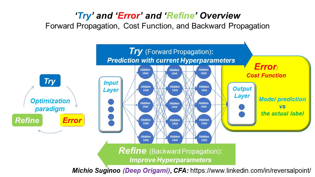
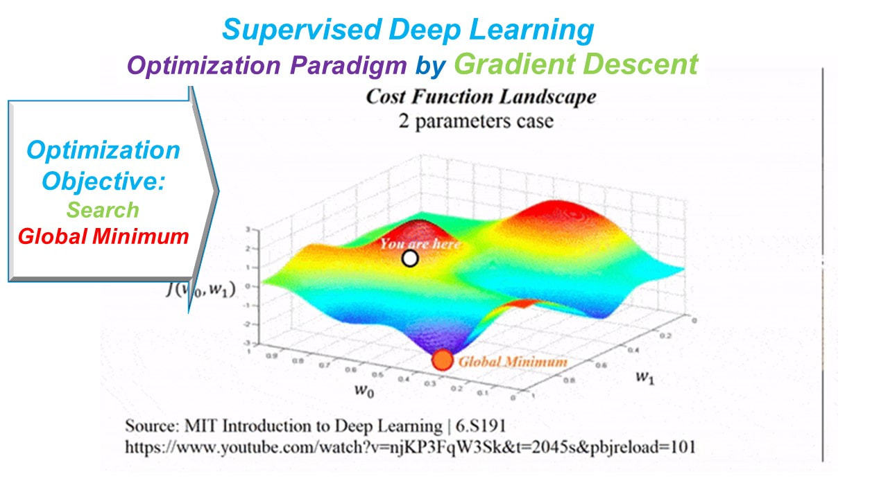
Chapter 4: Deep Learning’s Learning Mechanism
Optimization Paradigm driven by 3 Step Iteration Cycle

Originally published 16 February, 2021
By Michio Suginoo

In this chapter, we will have a quick look at the learning mechanism of Deep Learning.

How does it learn?

You can click on the video below.
Cut a long story short, Deep Learning is an optimization paradigm that learns through repetitions of “3 step Iteration Cycle”: Try and Error and Refine.

The next figure illustrates how this 3 step iteration cycle operates in the structure of “Feedforward Neural Networks”, a prototype of Deep Learning Algorithm, which you saw earlier.
Picture
The stack of layers in Deep Learning architecture is comprised of 3 functional sub-divisions: the input layer, the hidden layers, and the output layer.
 
Right after taking the input in the input layer, the model enters into the iteration cycle.
First, “prediction process” takes place in the hidden layers along “the blue arrow on the top”. The system tries the current values of Hyperparameters to generate a “tentative prediction”.

Then, second, “the measurement of the error” takes place in the yellow box. The output layer generates a tentative prediction based on the current values of hyperparameters. Thereafter, the network engages in the process of ‘Error’, using a Cost Function to measure the error between the current tentative prediction and the given actual labels.
  
Third, the refinement of hyperparameters takes place back in the hidden layers along the green arrow at the bottom. This process goes backward the way it came during the process of ‘Try’. So it is called Backward propagation.

And the system repeats this 3 step iteration cycle over and over, until it reduces the error within an acceptable range.

Overall, the hidden layers engage in two learning stages: to try the current values of hyperparameters in the process of ‘Try’; and to update the values of hyperparameters in the process of ‘Refine’.

Updating Hyperparameters

Next, let’ take a look at how the system refines the hyperparameter values.
The 3D chart here is a simplified illustration of the Cost Function.
Picture
Remember the ultimate objective of the optimization is to minimize the error, thus, the value of the cost function. In order to minimize the Error, we want to arrive at the bottom of the Cost Function Landscape in the illustration above.

Click the  animation video below. This illustrates the process of Deep Learning Optimization.
It’s like skiing along the downhill. This process is called Gradient Descent. Easier said than done. This chart is a little bit of over-simplification. The reality might be more complex. In Chapter 7, we will face the reality.

In the next chapter, we will have a quick look at the background behind Deep Learning Revolution in recent years.

Donation:
Please feel free to click the bottom below to donate and support
the activities of www.reversalpoint.com

​Copyright © by Michio Suginoo. All rights reserved.

Proudly powered by Weebly